Introduction to Biot-Savart Law and Understanding Magnetic Fields

Introduction to Biot-Savart Law

Introduction to Biot-Savart Law:

The Biot-Savart Law is a fundamental principle in electromagnetism that describes the magnetic field produced by a steady current in a wire. It was formulated by French physicists Jean-Baptiste Biot and Félix Savart in the early 19th century.

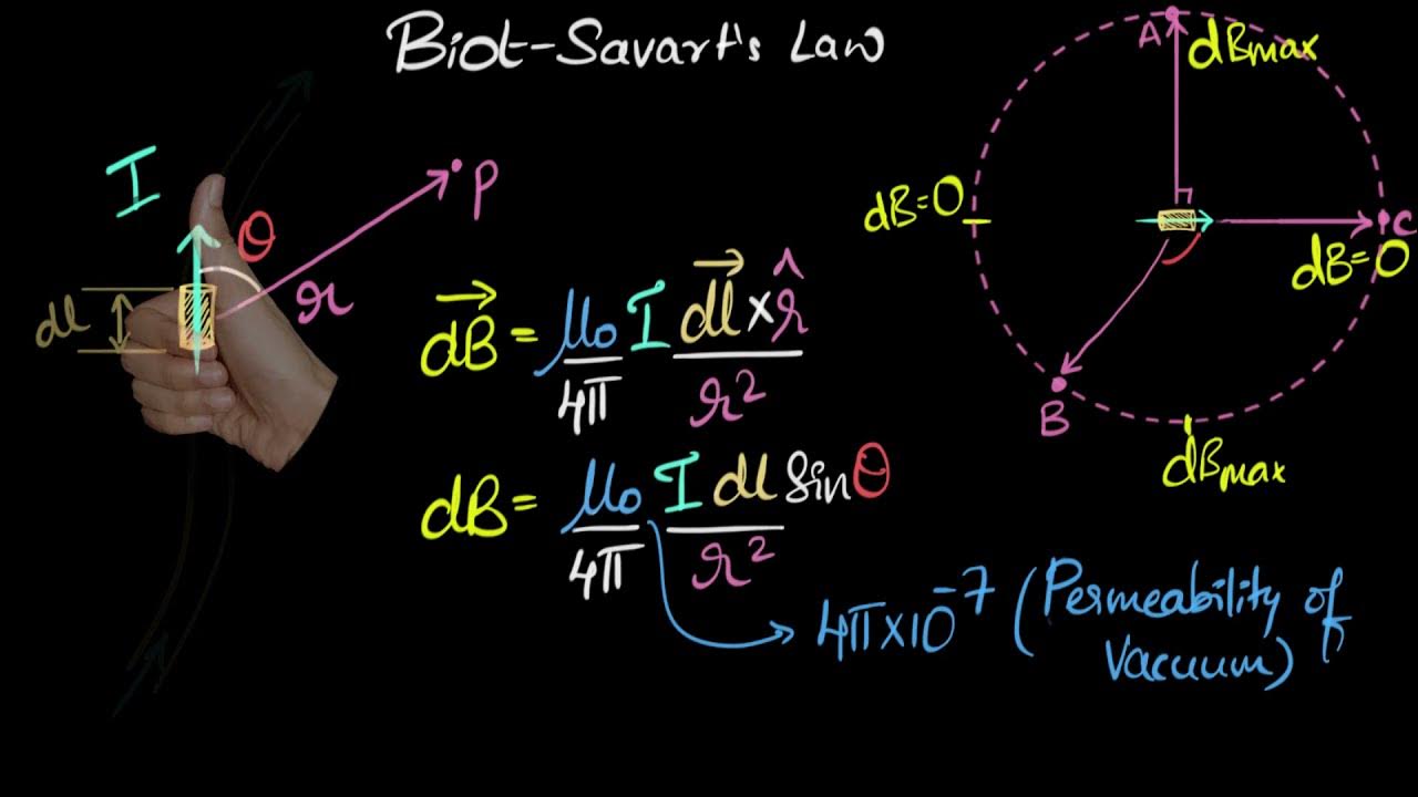
The law states that the magnetic field at a point in space due to a current-carrying segment of wire is directly proportional to the current, the infinitesimal length of the wire, and the sine of the angle between the wire and the line connecting the point to the wire. This relationship is given by the equation:

d𝐵 = (𝜇/4𝜋)(𝐼 d𝐿 × 𝐫)/𝑟²

where d𝐵 is the infinitesimal magnetic field produced at a point, 𝜇 is the permeability of free space, 𝐼 is the current in the wire, d𝐿 is the infinitesimal length element of the wire, 𝐫 is the vector connecting the element to the point in space, and 𝑟 is the distance between the element and the point.

By integrating the contributions from all the infinitesimal lengths of the wire, the total magnetic field produced by the whole wire can be determined at any given point. This law is applicable to both straight and curved wire segments.

The Biot-Savart Law is essential for understanding the behavior of magnetic fields generated by current-carrying conductors, such as wires, coils, and solenoids. It is widely used in various fields of physics and engineering, including electromagnetics, magnetostatics, and the design of electrical devices.

Overall, the Biot-Savart Law provides a mathematical framework to calculate the magnetic field produced by a current-carrying wire, offering valuable insights into the fundamental principles of electromagnetism.

Understanding Magnetic Fields

Understanding Magnetic Fields:

A magnetic field is a region in space where magnetic forces are exerted on charged particles or magnetic materials. It is generated by the movement of charged particles, such as electrons, or by permanent magnets. Magnetic fields are described by their strength, direction, and shape.

Magnetic fields have both magnitude and direction. The strength or intensity of a magnetic field is measured in units called Tesla (T) or Gauss (G), with 1 T equal to 10,000 G. The direction of the magnetic field is represented by lines called magnetic field lines. These lines form closed loops that indicate the direction in which a compass needle would point when placed in the magnetic field.

The magnetic field lines emerge from the North pole of a magnet and re-enter at the South pole. They are closer together near the poles, indicating a stronger field, and spread out farther away, indicating a weaker field. The interaction between magnetic fields and moving charged particles is what gives rise to phenomena like magnetism and electromagnetism.

Understanding Biot-Savart Law:

The Biot-Savart law is a mathematical formula that describes the magnetic field generated by a steady current-carrying wire. It was formulated by the French physicists Jean-Baptiste Biot and Félix Savart in the early 19th century.

According to the Biot-Savart law, the magnetic field (B) at a given point in space, due to a small length element (dL) of a current-carrying wire, is directly proportional to the product of the current (I), the length element (dL), and the sine of the angle (θ) between the length element and the line connecting the length element to the point.

Mathematically, the Biot-Savart law can be written as:

dB = (μ₀/4π) * (I * dL × r̂) / r²

Where dB is the magnetic field produced by the current element dL at a point in space, μ₀ is the permeability of free space (a constant), I is the current flowing through the wire, dL is an infinitesimally small element of the wire, r̂ is the unit vector pointing from the element to the point, and r is the distance between the length element and the point.

The Biot-Savart law provides a fundamental tool for calculating the magnetic field produced by different configurations of current-carrying wires or currents flowing in loops. It is essential in many areas of physics, including the study of electrical circuits, electromagnetism, and the behavior of magnetic materials.

Deriving the Biot-Savart Law

The Biot-Savart Law describes the magnetic field produced by a current-carrying wire. It is named after the French physicists Jean-Baptiste Biot and Félix Savart, who derived this law.

Consider a current-carrying wire with a current I flowing through it. We want to find the magnetic field at a point P that is a distance r away from the wire.

The magnetic field at point P can be determined by integrating the contributions of all infinitesimal elements of the wire.

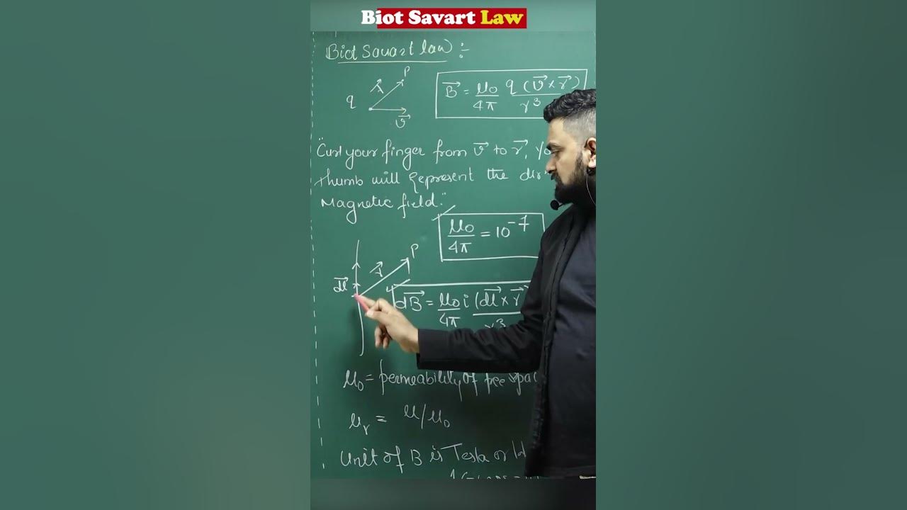
Let’s take an infinitesimal element of length dl on the wire and assume that it carries a current I’. The vector dl represents the direction and magnitude of the current element. The magnetic field produced by this current element at point P can be calculated using the following formula:

dB = (μ₀ / 4π) * (I’ * dl X r) / r²

In this equation, μ₀ is the permeability of free space, which is a constant value (approximately 4π x 10^-7 Tm/A). The term (I’ * dl X r) represents the cross product between the current element and the vector r, which points from the current element to the point P. The denominator r² accounts for the inverse square relationship between the distance and the magnetic field.

To find the total magnetic field at point P, we need to sum up the contributions from all the infinitesimal elements of the wire. This is done by integrating the equation over the entire length of the wire:

B = ∫ (μ₀ / 4π) * (I’ * dl X r) / r²

The integral is taken over the entire length of the wire.

The Biot-Savart Law provides a precise mathematical relationship between the current-carrying wire and the magnetic field it produces at a given point. It is a fundamental principle in electromagnetism and is widely used in various fields, including physics, engineering, and technology.

Applications of the Biot-Savart Law

The Biot-Savart law is a mathematical equation that describes the magnetic field produced by a steady current in a wire. It has numerous applications in various fields.

1. Electromagnetic induction: The Biot-Savart law is used to calculate the induced magnetic field in a closed path due to a changing current in a nearby wire or circuit. This principle is the basis for the operation of transformers, generators, and induction motors.

2. Magnetic field calculations: The law allows us to determine the magnetic field at any point in space produced by a current-carrying wire. This is useful in designing electromagnets and understanding the magnetic behavior of materials.

3. Magnetic field of a current loop: By using the Biot-Savart law, we can calculate the magnetic field at any point on the axis of a circular loop carrying a steady current. This is used in practical applications such as magnetic compasses and MRI scanners.

4. Ampere’s law: The Biot-Savart law serves as the basis for deriving Ampere’s law, which relates the magnetic field around a closed loop to the current enclosed by the loop. Ampere’s law is used to calculate the magnetic field produced by symmetric current distributions and is essential in solving problems in electromagnetism.

5. Electrical engineering: In the design and analysis of electrical devices and circuits, the Biot-Savart law is often used to calculate the magnetic field produced by current-carrying conductors. This is helpful in determining the forces experienced by conductors in magnetic fields and in analyzing the performance of electrical machines like motors and generators.

Overall, the Biot-Savart law is a fundamental principle in electromagnetism, and its applications are widespread in various disciplines including physics, electrical engineering, and medical imaging.

Limitations and Extensions of the Biot-Savart Law

The Biot-Savart law is a mathematical equation that describes the magnetic field generated by a current-carrying wire. However, like any scientific law, it has its limitations and can be extended for certain cases.

1. Steady-State Currents: The Biot-Savart law applies to steady-state currents, where the current does not change with time. It does not accurately describe the magnetic field produced by changing currents or transient phenomena.

2. Infinite Current Elements: The Biot-Savart law assumes that the current is distributed uniformly along an infinitely long and thin wire. In reality, actual wires have finite lengths and thicknesses, which may cause deviations from the predicted magnetic field.

3. Magnetic Field Calculations: The Biot-Savart law provides a calculation for the magnetic field at a single point in space due to a current element. To find the magnetic field produced by a current-carrying wire with a complex shape, such as a loop or a coil, the law needs to be applied at several points and integrated numerically.

Extensions:

1. Ampere’s Law: Ampere’s law is an extension of the Biot-Savart law. It states that the magnetic field around a closed loop is directly proportional to the current passing through the loop. Ampere’s law is a more convenient tool to calculate magnetic fields in cases of symmetry, such as long straight wires or circular loops.

2. Magnetic Field Due to Discrete Current Elements: The Biot-Savart law can be extended to calculate the magnetic field produced by a system of discrete current elements. By summing the contributions from each element, the total magnetic field can be determined.

3. Magnetic Field Due to Permanent Magnets: The Biot-Savart law can also be extended to describe the magnetic fields produced by permanent magnets. In this case, the magnetic field is determined by the sum of the individual magnetic moments of the atoms or domains within the material.

In summary, while the Biot-Savart law provides a fundamental equation for calculating magnetic fields due to steady-state currents, it has limitations such as its applicability to infinite current elements and steady-state currents only. However, it can be extended for different scenarios like calculating magnetic fields using Ampere’s law and considering discrete current elements or permanent magnets.

Topics related to Biot-Savart Law