Introduction to Kalman Filter in mathematics and Basic principles of Kalman Filter

Introduction to Kalman Filter in mathematics

The Kalman filter is a mathematical tool used in the field of signal processing and control systems to estimate the state of a dynamic system. It was developed by Rudolf Kalman in the 1960s and has found applications in a wide range of fields such as aerospace, robotics, economics, and weather forecasting.

At its core, the Kalman filter is a recursive algorithm that takes in noisy measurements of a system’s output and produces an optimal estimate of its true state, based on a mathematical model of the system dynamics. It combines information from both the measurements and the model predictions to improve the accuracy and reliability of the state estimation.

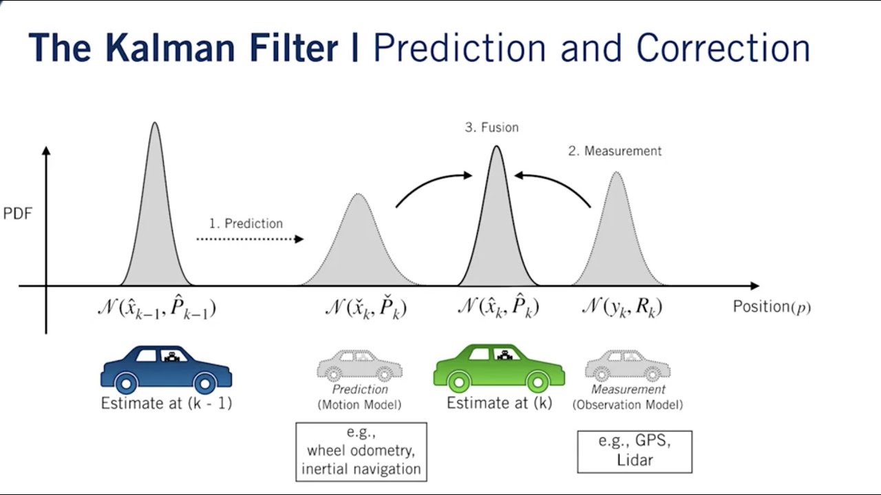
The filter works by maintaining two estimates of the system state: the prior estimate, which is based on the previous estimate and the model prediction, and the posterior estimate, which is updated using the measurements. The Kalman filter also calculates the error covariance matrix, which provides a measure of the estimation uncertainty.

The key idea behind the Kalman filter is that it uses a weighted average of the prior and posterior estimates as the final estimate, with the weights determined by the uncertainty associated with each estimate. The filter dynamically adjusts these weights using a process known as the Kalman gain, which minimizes the mean square error between the estimated and true states.

Overall, the Kalman filter is highly effective in dealing with noisy measurements and can handle systems with complex dynamics and non-linearities. It provides an efficient and robust solution for state estimation problems, making it a widely used tool in various fields of science and engineering.

Basic principles of Kalman Filter

The Kalman Filter is a widely used mathematical algorithm that is used to estimate the state of a dynamic system based on incomplete and noisy measurements. It provides a recursive solution to the problem of state estimation and is often used in control systems, navigation systems, signal processing, and many other applications.

Here are some basic principles of the Kalman Filter:

1. Linear Gaussian model: The Kalman Filter assumes that the dynamic system and measurement model are both linear and that the noises in the system follow Gaussian distributions.

2. State and measurement models: The system being estimated is described by a state vector that evolves over time according to a linear dynamical system model. The measurements are obtained from the system and are related to the state through a linear measurement model.

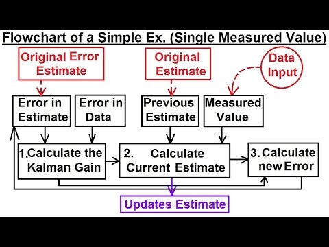
3. Prediction step: The Kalman Filter predicts the current state based on the previous state estimate and the system model. It also predicts the error covariance, which represents the uncertainty in the state estimate.

4. Update step: The prediction is then corrected based on the measurements obtained. This is done by comparing the predicted measurement with the actual measurement and adjusting the state estimate and error covariance accordingly.

5. Optimal estimate: The Kalman Filter provides an optimal estimate of the state by minimizing the mean square error between the estimated state and the true state.

6. Recursive nature: The Kalman Filter operates in a recursive manner, meaning that it continuously updates and refines the state estimate as new measurements become available. It maintains the current state estimate and the error covariance, and uses them as inputs for the next prediction and update steps.

These principles form the foundation of the Kalman Filter algorithm and allow it to provide accurate and efficient estimation of the state of dynamic systems even in the presence of noise and uncertainty.

Mathematical formulation of Kalman Filter

The Kalman Filter is a mathematical model used to estimate states of dynamic systems by combining measured data with predictions from a system model. It is commonly used in control systems, signal processing, and navigation applications.

The mathematical formulation of the Kalman Filter consists of two main steps: prediction and update.

1. Prediction Step:

– State Prediction: x̂(k) = Fx(k-1) + Bu(k) + w(k)

– x̂(k): predicted state at time k

– F: state transition matrix

– x(k-1): previous state at time k-1

– B: control input matrix

– u(k): control input at time k

– w(k): process noise

– Covariance Prediction: P(k) = F P(k-1) F^T + Q

– P(k): predicted covariance at time k

– Q: process noise covariance matrix

2. Update Step:

– Innovation or Measurement Residual: y(k) = z(k) − H x̂(k)

– y(k): measurement residual at time k

– z(k): measured output at time k

– H: measurement matrix

– Innovation Covariance: S(k) = H P(k) H^T + R

– S(k): innovation covariance at time k

– R: measurement noise covariance matrix

– Kalman Gain: K(k) = P(k) H^T S(k)^−1

– K(k): optimal Kalman gain at time k

– State Update: x(k) = x̂(k) + K(k) y(k)

– x(k): updated state at time k

– Covariance Update: P(k) = (I − K(k) H) P(k)

– I: identity matrix

In summary, the Kalman Filter predicts the state of a system based on the previous state and control inputs, taking into account the process noise. It then compares the predicted state with the measured output and calculates the discrepancy or innovation. Using the innovation, measurement and process noise covariance matrices, it determines the Kalman gain that balances the importance of the predicted state and the measured output. Finally, the Kalman gain is used to update the state and covariance estimates.

Applications of Kalman Filter

The Kalman filter is a widely used mathematical technique that can be applied to a variety of applications to estimate the state of a dynamic system. Some common applications of the Kalman filter include:

1. Navigation and tracking: The Kalman filter can be used to estimate the position, velocity, and other states of a moving object based on noisy sensor measurements, such as GPS or radar data. It is widely used in autonomous vehicles, aircraft navigation, and mobile robotics.

2. Robotics: The Kalman filter is used for state estimation in robotics to estimate the position and orientation of the robot using sensor measurements from cameras, range finders, and IMUs. It helps in localizing the robot accurately even in the presence of noise and uncertainty.

3. Financial forecasting: The Kalman filter can be used to model and forecast financial time series data, such as stock prices or exchange rates. It allows for the incorporation of noisy observations and provides a more accurate prediction of the future financial states.

4. Signal processing: It is used in signal processing applications, such as speech recognition, image processing, and video tracking. The Kalman filter helps in denoising the signals and tracking the features of interest in real-time.

5. Control systems: The Kalman filter is extensively used in control systems to estimate the state of a dynamic system based on noisy sensor measurements. It is used in applications such as flight control systems, process control in manufacturing, and robotic manipulators to provide accurate feedback for control.

6. Weather forecasting: The Kalman filter can be used in weather prediction models to estimate the state variables, such as temperature, humidity, and wind speed, based on noisy sensor observations. It helps improve the accuracy of weather forecasts by assimilating real-time observations.

7. Biomedical engineering: The Kalman filter is employed in various biomedical applications, such as electrocardiogram (ECG) signal processing, respiratory monitoring, and blood glucose estimation. It assists in removing noise, artifacts, and estimation of the physiological states accurately.

Overall, the Kalman filter finds its applications in a wide range of fields where accurate estimation and state prediction are crucial in the presence of noisy measurements and uncertainties.

Advantages and limitations of Kalman Filter

Advantages of Kalman Filter:

1. Kalman Filter is an optimal estimation algorithm, which means it provides the most accurate estimate of the state of a system.

2. It can handle noisy measurements and uncertain system dynamics, leading to robust and accurate state estimation.

3. It is computationally efficient and can be implemented in real-time applications.

4. Kalman Filter can handle non-linear system models by using an extended version called Extended Kalman Filter (EKF).

5. It can model and track multiple objects simultaneously using multi-object tracking extensions.

6. It has a solid theoretical foundation and well-established mathematical properties.

Limitations of Kalman Filter:

1. It assumes that the system is linear and that the noise is Gaussian, which may not hold true in certain real-life scenarios.

2. Kalman Filter requires knowledge of the system dynamics and measurement models, including the noise covariance matrices, which can be challenging to estimate accurately.

3. It assumes that the system is observable, meaning that it is possible to estimate the state from the available measurements. In certain cases, the system may not be fully observable, leading to inaccurate results.

4. It is sensitive to the initial state estimation and assumptions about the noise statistics.

5. Kalman Filter can struggle with handling abrupt changes or outliers in measurements, as it assumes a smooth transition between states.

6. It can be challenging to tune the filter parameters appropriately for optimal performance.

Topics related to Kalman Filter