Introduction to the Black-Scholes Equation
The Black-Scholes equation is a mathematical model that is widely used in the field of financial physics to price options contracts. It was developed by economists Fischer Black and Myron Scholes in 1973 and has since become a cornerstone of modern financial theory.
In simple terms, the Black-Scholes equation is used to calculate the fair value of an options contract, which gives the right but not the obligation to buy or sell an underlying asset at a predetermined price (the strike price) within a specified period of time. This equation takes into account various factors including the current price of the underlying asset, the strike price, the time remaining until expiration, and the volatility of the asset’s price.
The equation assumes that financial markets are efficient and that the price of the underlying asset follows a geometric Brownian motion, meaning that its value changes randomly over time. It also assumes that there are no transaction costs, no dividends paid on the underlying asset, and that interest rates are constant.
The Black-Scholes equation is a partial differential equation that can be solved using various mathematical techniques such as the method of separation of variables or the use of stochastic calculus. By solving the equation, one can determine the theoretical fair value of an options contract. This value can then be compared to the market price of the option to determine whether it is overpriced, underpriced, or fairly valued.
Despite its widespread use, the Black-Scholes equation has certain limitations and assumptions that may not hold in real-world financial markets. These include the assumption of constant volatility, which is not always accurate, and the assumption of continuous trading, which may not be practical in certain situations. These limitations have led to the development of more advanced models, such as the Heston model and the SABR model, which aim to overcome some of these shortcomings.
Overall, the Black-Scholes equation remains a valuable tool in financial physics for pricing options contracts and understanding the dynamics of financial markets. Its elegant mathematical formulation has had a significant impact on the field of finance and continues to be a topic of study and research.
Overview of Financial Physics
Financial Physics is a multidisciplinary field that applies principles and methods from physics to understand and analyze financial markets and economic systems. It aims to model and predict the behavior of financial markets using mathematical and computational techniques.
One of the fundamental concepts in financial physics is the Black-Scholes equation, which is a partial differential equation used to price options and derivatives. It was developed by economists Fischer Black and Myron Scholes in 1973, and later refined by Robert C. Merton.
The Black-Scholes equation is derived from the assumption that financial markets follow a geometric Brownian motion, meaning that the prices of assets fluctuate randomly over time. It takes into account factors such as the current price of the underlying asset, the strike price of the option, the time until expiration, the risk-free interest rate, and the volatility of the underlying asset.
The equation is expressed as:
∂V/∂t + 1/2 σ^2 S^2 ∂^2V/∂S^2 + r S ∂V/∂S – rV = 0
where:
V is the price of the option or derivative,
t is time,
S is the price of the underlying asset,
σ is the volatility of the underlying asset,
r is the risk-free interest rate.
The equation provides a mathematical framework to calculate the fair value of options and derivatives and to hedge against market risks. It allows traders and investors to determine the optimal prices to buy or sell options, given the current market conditions and expected volatility.
The use of the Black-Scholes equation in financial physics extends beyond pricing options. It allows researchers to analyze and understand the dynamics and behavior of financial markets, studying phenomena such as market efficiency, risk management, and the impact of various factors on prices and trading strategies.
Overall, the Black-Scholes equation plays a crucial role in financial physics by providing a mathematical foundation for pricing options and derivatives and aiding in the analysis and modeling of financial markets.
Derivation and Components of the Black-Scholes Equation
The Black-Scholes equation is a mathematical model used in financial physics to estimate the price of options. It was developed by economists Fischer Black and Myron Scholes in 1973.
Derivation of the Black-Scholes Equation:
The derivation of the Black-Scholes equation is based on assumptions about the market, including efficient market theory, constant risk-free interest rates, and continuously tradable assets. The main idea behind the derivation is to create a risk-neutral portfolio by combining the option with the underlying asset in such a way that the portfolio’s value does not depend on the future price movements of the asset.
Components of the Black-Scholes Equation:
The Black-Scholes equation contains several components that contribute to the calculation of option prices. These components are:
1. Stock Price (S): The current market price of the underlying asset (e.g., a stock).
2. Strike Price (K): The predetermined price at which the option can be exercised.
3. Time to Expiration (T): The remaining time until the option’s expiration date.
4. Risk-Free Interest Rate (r): The rate of return that can be obtained from a risk-free investment.
5. Volatility (σ): A measure of the asset’s price fluctuations over time.
6. Dividend Yield (δ): The rate at which the asset pays dividends (if applicable).
The Black-Scholes equation combines these components to estimate the fair price of a European call or put option. It assumes that the underlying asset follows a geometric Brownian motion, meaning its price changes randomly but follows a specific pattern.
The equation mathematically describes the relationship between the option price and the various components mentioned above. It is a partial differential equation that can be solved to determine the fair value of the option at any given time.
The Black-Scholes equation has significantly contributed to the field of financial physics by providing a framework for pricing options and understanding their dynamics in the market.
Applications of the Black-Scholes Equation in Finance
The Black-Scholes equation is a mathematical model used in finance to calculate the price of options. In the context of financial physics, it is a partial differential equation that describes the behavior of financial instruments, such as stock options, and their underlying assets, including stocks and commodities.
Here are some important applications of the Black-Scholes equation in finance:
1. Option pricing: The Black-Scholes equation is primarily used for pricing options. By inputting the relevant parameters such as the underlying asset price, strike price, time to expiration, volatility, and risk-free interest rate, the equation can determine the fair value of an option. This enables investors to make informed decisions about buying, selling, or hedging options.
2. Risk management: The Black-Scholes equation allows financial institutions to analyze and manage their risk exposure associated with derivatives, such as options. By employing the model, they can assess the sensitivity of option prices to changes in underlying asset prices, volatility, and other factors. This information helps in designing risk management strategies to protect against adverse market movements.
3. Implied volatility estimation: The Black-Scholes equation can be used to estimate implied volatility, which is a measure of market expectations about future price moves. By plugging in the option price and other known parameters, the equation can be solved iteratively to find the implied volatility level that matches the observed market price. Implied volatility is a crucial input for option trading and risk management strategies.
4. Option Greek calculations: The Black-Scholes equation provides a framework for calculating various derivative sensitivities, commonly known as “Greeks.” These include delta (sensitivity to the underlying asset’s price), gamma (sensitivity of delta to changes in the underlying asset price), theta (time decay), vega (sensitivity to changes in volatility), and rho (sensitivity to changes in interest rates). These Greeks are essential for understanding and managing the risk and performance of options portfolios.
5. Volatility forecasting: Financial physicists and quantitative analysts use the Black-Scholes equation to develop models for forecasting future volatility. By analyzing historical option prices and solving the equation backward, they can estimate the implied volatility dynamics and project future volatility levels. These forecasts are crucial for pricing complex options, designing trading strategies, and managing portfolio risk.
Overall, the Black-Scholes equation forms the foundation of modern option pricing theory and provides valuable insights and tools for the practice of financial physics in finance. It has revolutionized the way options are priced, traded, and managed, and has played a significant role in the development of quantitative finance.
Critiques and Limitations of the Black-Scholes Equation
The Black-Scholes equation, also known as the Black-Scholes-Merton model, is widely used in financial markets to estimate the price of options. While it has been incredibly influential in the field of quantitative finance, it is important to recognize its critiques and limitations. Here are a few:
1. Assumptions: The Black-Scholes equation is built upon several key assumptions, including constant volatility, efficient market hypothesis, no transaction costs, continuous trading, and no dividend payouts. These assumptions do not always hold true in real-world financial markets, limiting the applicability of the equation.
2. Volatility assumption: The Black-Scholes equation assumes that the volatility of the underlying asset is constant. However, in reality, volatility can change over time, leading to potential inaccuracies in option pricing.
3. Market frictions: The Black-Scholes equation neglects market frictions such as transaction costs and liquidity constraints. These frictions can significantly impact the actual prices of options, rendering the equation less reliable in real-world scenarios.
4. Normal distribution assumption: The Black-Scholes equation assumes that the distribution of asset returns is normally distributed. However, empirical evidence suggests that asset returns often exhibit skewness and kurtosis, meaning that the actual distribution deviates from the normal distribution assumption.
5. Risk-neutral valuation: The Black-Scholes equation uses the risk-neutral valuation approach, assuming that investors are indifferent to risk. This may not accurately reflect the behavior of real investors, who often have risk preferences that vary from the risk-neutral stance.
6. Lack of consideration for market dynamics: The Black-Scholes equation does not take into account market dynamics such as market crashes, high-frequency trading, or other time-dependent effects. These dynamics can have a substantial impact on option prices and cannot be captured by the equation alone.
In the context of financial physics, where the Black-Scholes equation is explored from a broader scientific perspective, additional criticisms and limitations arise. These include:
1. Psychological and behavioral factors: The Black-Scholes equation assumes rational behavior and does not consider psychological and behavioral elements that can influence market dynamics and option prices. Financial physics seeks to incorporate these factors into the equation to provide a more realistic representation of the market.
2. Agent-based modeling: Financial physics explores agent-based modeling techniques to capture the interactions and behaviors of market participants. This approach goes beyond the assumptions made in the Black-Scholes equation, allowing for a more nuanced understanding of market dynamics.
3. Complexity and higher-order effects: Financial physics acknowledges that financial markets are complex systems with interdependencies and higher-order effects that are not fully captured by the Black-Scholes equation. It strives to develop models that incorporate these complexities for better predictions and risk management.
In summary, while the Black-Scholes equation has been widely used in finance for option pricing, it has its critiques and limitations. These include assumptions that may not hold true in real-world scenarios, neglect of market frictions, limitations in volatility estimation, and the failure to capture the dynamic nature of markets. Financial physics seeks to address some of these limitations by incorporating psychological factors, agent-based modeling, and a recognition of market complexity.
Topics related to Black-Scholes Equation (in the context of financial physics)
19. Black-Scholes Formula, Risk-neutral Valuation – YouTube

19. Black-Scholes Formula, Risk-neutral Valuation – YouTube
The Easiest Way to Derive the Black-Scholes Model – YouTube

The Easiest Way to Derive the Black-Scholes Model – YouTube
A simple derivation of the Black-Scholes equation – YouTube

A simple derivation of the Black-Scholes equation – YouTube
QUANT FINANCE 1 – Why We Never Use the Black Scholes Equation, 1 – YouTube

QUANT FINANCE 1 – Why We Never Use the Black Scholes Equation, 1 – YouTube
Black Scholes Formula I – YouTube

Black Scholes Formula I – YouTube
Black-Scholes Equation from Ito's Lemma – YouTube
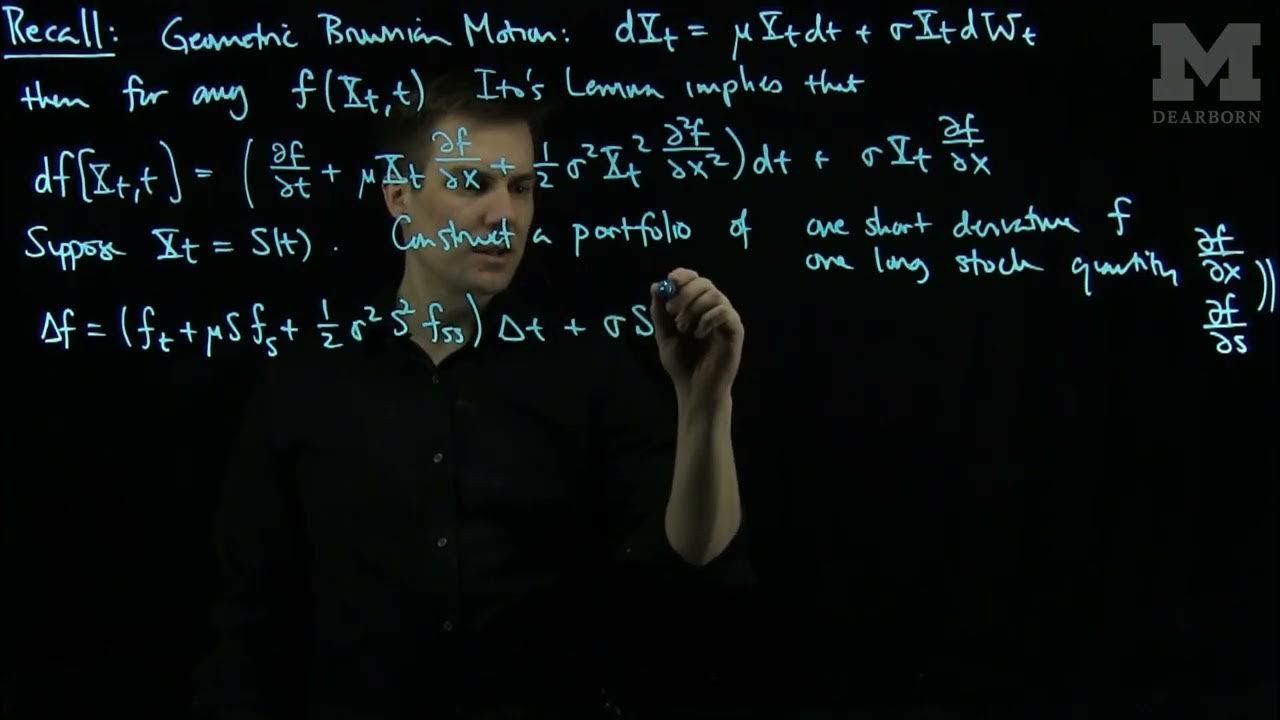
Black-Scholes Equation from Ito's Lemma – YouTube
KASNEB-CPA-Financial Management-BLACK SCHOLES OPTION MODEL – YouTube

KASNEB-CPA-Financial Management-BLACK SCHOLES OPTION MODEL – YouTube
Black-Scholes PDE Derivation in 4 minutes – YouTube

Black-Scholes PDE Derivation in 4 minutes – YouTube
Live Solve of the 2023 AMC 12B unseen, 75 minute solve – YouTube

Live Solve of the 2023 AMC 12B unseen, 75 minute solve – YouTube
La formule qui a radicalement transformé la finance mondiale [Black-Scholes] – YouTube

La formule qui a radicalement transformé la finance mondiale [Black-Scholes] – YouTube

Konstantin Sergeevich Novoselov is a Russian-British physicist born on August 23, 1974. Novoselov is best known for his groundbreaking work in the field of condensed matter physics and, in particular, for his co-discovery of graphene. Novoselov awarded the Nobel Prize in Physics. Konstantin Novoselov has continued his research in physics and materials science, contributing to the exploration of graphene’s properties and potential applications.